Image Segmentation with Graph Cuts
By JULIE JIANG
Update in 2022: This project was done as a class project for an algo class when I was an undergrad at Tufts University in 2017, back when I knew next to nothing about rigorous research methodologies and academic writing. Over the years, this project has surprisingly attracted some attention, therefore I've minimally edited this page to correct for grammar mistakes and typos. Enjoy! -Julie
Intro
Graph algorithms have been successfully applied to a number of computer vision and image processing problems. Our interest is in the application of graph cut algorithms to the problem of image segmentation.
This project focuses on using graph cuts to divide an image into background and foreground segments. The framework consists of two parts. First, a network flow graph is built based on the input image. Then a max-flow algorithm is run on the graph in order to find the min-cut, which produces the optimal segmentation.
Network Flow
A network flow $G=(V,E)$ is a graph where each edge has a capacity and a flow. Two vertices in the network flow are designated to be the source vertex $s$ and the sink vertex $t$, respectively. The goal is to find the maximum amount of flow that could be delivered from $s$ to $t$, while satisfying the following constraints.
- Capacity constraint: Each edge $(u,v)\in E$ has a nonnegative capacity $c(u,v)$ that must be greater than or equal to its flow $f(u,v)$. $$0\leq f(u,v)\leq c(u,v)$$
- Flow conservation: For all vertices $u\in V-{s,t}$, we require that the inflow of the vertex is equal to its outflow. $$\sum_{v\in V}f(v,u)=\sum_{v\in V}f(u,v)$$ But $s$ can have unlimited inflow, and $t$ can have unlimited outflow.
The flow of the network is the flow that can be sent through some path from $s$ to $t$, which, by conservation of flow, is equal to the inflow of $s$ or the outflow of $t$. An $s/t$ cut is a partitioning of the vertices into two disjoint subsets such that one contains $s$ and the other contains $t$. The value of an $s/t$ cut is the total flow of the edges passing through the cut.
As stated by the max-flow min-cut theorem, the maximum amount of flow passing from the source to the sink is equivalent to the net flow of the edges in the minimum cut. So by solving the max-flow problem, we directly solve the min-cut problem as well. We will discuss algorithms for finding the max-flow or min-cut in a later section.
Image to Graph
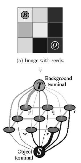
One of the most challenging things about this project is how to transform an image into a graph. In Graph cuts and efficient N-D image segmentation by Boykov and Funka-Lea, the authors described in great detail how to define a graph based on an image. Our implementation closely follows their idea of constructing the graph. For simplicity, we will use grayscale square images. Although the same idea could be easily extended to colored images with a suitable inter-pixel similarity measurement and also to rectangular images.
In this image-graph transformation scheme, a pixel in the image is a vertex in the graph labeled in row-major order. These vertices are called pixel vertices. In addition, there are two extra vertices that serve as the (invisible) source and the sink.
There are two types of edges in our graph. The first type is an $n$-link, which connects neighboring pixel vertices in a 4-neighboring system. The second type of edge is called a $t$-link. $t$-links connect the source or sink vertex with the pixel vertices.
The $n$-link edges must have weights carefully computed in order to reflect inter-pixel similarities. Concretely, we want the weight of an edge to be large when the two pixels are similar, and small when they are quite different. One idea is to compute the weight from a boundary penalty function that maps two pixel intensities to a positive integer. Let $I_p$ be the brightness, or intensity, of the pixel vertex $p$. For any edge $(p,q)\in E$, the boundary penalty $B(I_p, I_q)$ is defined as: $$ B(I_p, I_q) = 100\cdot \exp\Bigg(\frac{-(I_p-I_q)^2}{2\sigma ^2}\Bigg)$$.
This choice of $\sigma$ is determined from a series of trial and error. The penalty is high if $|I_p-I_q|<\sigma$, and is quite negligible if $|I_p-I_q|>\sigma$. From empirical results, we choose $\sigma=30$. Finally, the result is multiplied by 100 and cast to an integer. This is because network flow models require that the capacities be discrete rather than continuous.
To facilitate the model to make suitable $t$-links, the user is prompted to highlight at least one pixel vertex as a background pixel and at least one as a foreground pixel. These pixel vertices are called seeds. For every background seed, an edge is added from the source vertex to the background seed with capacity $\mathcal{K}$ defined as follows. $$ \mathcal {K} = \max(\{B(I_p, I_q)|(p, q)\in E\}) $$ In a similar fashion, edges to the sink vertex are added for every foreground seeds with capacity $\mathcal{K}$.
As these seeds share an edge with the source or sink vertices, they are hard-coded to be either the foreground or the background.
Now with the graph fully defined, we can run a graph cut algorithm to find the maximum flow/minimum cut.
Algorithms
There are several algorithms for finding the maximum flow/minimum cut. This project explores the efficiency of the Edmonds-Karp algorithm and the push-relabel algorithm. Though these are very standard and straightforward algorithms, we caution that they are often slow in practice.
Edmonds-Karp Algorithm
The Edmonds-Karp algorithm is an implementation of the Ford-Fulkerson method. First, we define a residual network $G_f=(V,E_f)$ to be the same network but with capacity $c_f(u,v)=c(u,v)-f(u,v)$ and no flow. The idea behind the Ford-Fulkerson method is that if there exists a path from $s$ to $t$ in the residual network, then we can augment the current flow by this path. This path is called the augmenting path. The augmentation of this path is equal to the smallest residual capacity along this path. Once no augmenting path can be found, the current flow must be the max-flow.
while there is a path from s to t in the residual network:
    flow = min([residual capacity of every edge along this path])
    for every edge (u,v) in this path:
        residual capacity of (u,v) -= flow
        residual capacity of (v,u) += flow
The Ford-Fulkerson method is called a method and not an algorithm because it does not specify how one should go about finding the augmenting path. The Edmonds-Karp algorithm specifies that the Ford-Fulkerson method be carried out via a breadth-first search to find a viable path in every iteration.
Since we are interested in the min-cut, we add one additional step after the main loop. According to the definition of the $s/t$ cut, $S$ contains the set of vertices reachable from $s$ in the residual network and $T$ contains the rest of the vertices. Therefore, we can run a depth-first search from $s$ using the residual network and deduce which edges are cut.
The Edmonds-Karp algorithm is an $O(VE^2)$ algorithm. An augmenting path can be found in $O(E)$, and the length of such path is $O(V)$. Since in every iteration, at least one edge becomes fully saturated, the number of times the same path is found to be the augmenting path is $O(V)$. This means the total number of times we can find an augmenting path is bounded by $O(VE)$. The body of the while loop runs in $O(E)$ time, so in total the time complexity is $O(VE^2)$. An accessible proof can be found in CLRS.
Push Relabel Algorithm
In the Push Relabel algorithm, we maintain a "preflow", which is a flow sent through the network but does not necessarily satisfy the flow conservation. In a preflow, the flow entering a vertex can be larger than the flow exiting the vertex. Given a preflow, a vertex can have an excess flow equal to the difference between the flow entering the vertex and the flow exiting the vertex. A vertex with excess flow is called an overflowing vertex.
In addition, we augment each vertex with a height attribute. Let $h(u)$ denote the height of a vertex u. The heights determine how a flow can be pushed. We can only push a flow from a higher vertex to a lower vertex, and not the other way around.
We start off by saturating all outgoing edges from $s$. This produces a valid preflow. We also set the height of $s$ to be the number of vertices. All other heights are set to 0. The algorithm centers around two main operations: push and relabel. For a given vertex $u$, we can push it by finding an outgoing edge from $u$ that is not saturated. The push to this edge is equal to the minimum of the residual capacity of the edge and the excess flow of $u$. Once the flow is pushed, the excess flow at $u$ falls by the amount of the pushed flow, and the excess flow at $v$ increases by the same amount. Not all edges can be pushed, however. In that case, we will relabel $u$ by setting the height of $u$ to be $$h(u)=1+\min\{h(v)|(u,v)\in E_f\}$$
while there exists an overflowing vertex u:
    push(u) or relabel(u)
The Push Relabel algorithm runs in $O(V^2E)$ time, improving upon the Edmonds-Karp algorithm. We prove this by bounding the number of times a vertex can be found overflowing.
Usage
The source code is available for download at https://github.com/julie-jiang/image-segmentation/. Make sure you have the following dependencies installed:
- Python 2 or 3
- OpenCV for python
- NumPy
To run the program, provide a JPG image and run
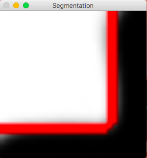
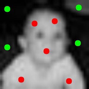
$ python imagesegmentation.py yourImage.jpgA window will soon pop up prompting you to plant object (foreground) seeds. Use your cursor to mark points or draw lines on the window to label any part of the graph as foreground. Once you're done, press ESC to continue. A second window will now pop up prompting you to plant background seeds. As with before, press ESC to continue. In about half a minute, the resulting image segmented image will be shown. Press ESC when you're ready to quit the program. The seeded image and the segmented image will both be saved.


The program uses the Edmonds-Karp algorithm by default. To use the Push-Relabel algorithm, add the flag --algorithm pr .
Limitations
As the size of the network flow graph grows quadratically with the size of the input image, the program should only be used on very small images. Empirically, we found that the program runs reasonably fast (under a minute) on an image of size 30x30 pixels. Therefore, all input images will be resized to 30x30 at the beginning of the program. The following example images look big because bigger images are easier on the eyes and also because marking pixels using OpenCV is only accurate when the image is big enough. All images are sized up before being displayed or saved.
Furthermore, the program may fail to identify the correct cuts. For example, if there isn't sufficient seeds, then the program may only cut between the source/sink vertex and the pixel vertices--corresponding to no visible cuts in our image--or it may try to cut only around the seeds. One solution is to increase the number of seeds. Another method, introduced by Shi and Malik in Normalized Cuts and Image Segmentation, uses normalized cuts to penalize cuts that only partition a small localized region of the image.
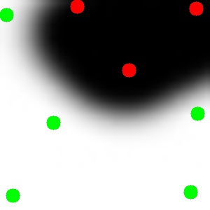
Results
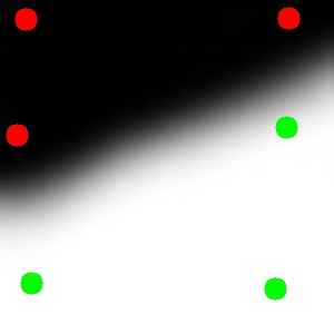
The following is a series of seeded images and the resulting segmentations.


References
- Boykov, Yuri, and Gareth Funka-Lea. Graph cuts and efficient ND image segmentation." International journal of computer vision 70, no. 2 (2006): 109-131.
- Boykov, Yuri Y., and M-P. Jolly. "Interactive graph cuts for optimal boundary & region segmentation of objects in ND images." In Computer Vision, 2001. ICCV 2001. Proceedings. Eighth IEEE International Conference on, vol. 1, pp. 105-112. IEEE, 2001.
- Boykov, Yuri, and Vladimir Kolmogorov. "An experimental comparison of min-cut/max-flow algorithms for energy minimization in vision." IEEE transactions on pattern analysis and machine intelligence 26, no. 9 (2004): 1124-1137.
- Shi, Jianbo, and Jitendra Malik. "Normalized cuts and image segmentation." IEEE Transactions on pattern analysis and machine intelligence 22, no. 8 (2000): 888-905.
- Eriksson, Anders P., Olof Barr, and Kalle Astrom. "Image segmentation using minimal graph cuts." (2006).
- Felzenszwalb, Pedro F., and Daniel P. Huttenlocher. "Efficient graph-based image segmentation." International journal of computer vision 59, no. 2 (2004): 167-181.